How to Optimize Amazon Redshift Performance

Amazon Redshift is a fully managed, petabyte-scale data warehouse that enables companies to quickly consolidate and analyze their data using a data analytics solution. In running complex queries against large amounts of data within your Amazon Redshift data warehouse, it can be taxing on the overall system.

It’s important to apply best practices and resolve optimization issues fast, because the longer you wait, the fewer real-time insights you’ll have access to and the more deep debugging awaits you in the future. This post will take you through the most common issues Amazon Redshift users come across, and will give you advice on how to address each of those issues.

Remember, even one inefficient query can cause performance issues, so let’s tackle them early and often. And once you’ve resolved your inefficient queries and reinstated optimal Amazon Redshift performance, you can continue real-time data analytics and drive your business forward.

1. Time Consuming Queries

When monitoring the performance of the database, one the most important things you want to keep track of are basic statistics regarding execution time. With the following query, you can monitor the most time consuming queries along with the average, minimum and maximum execution time. Knowing which queries are most problematic is the first step in debugging the situation. Then, you can dive deeper trying to determine the reason why these queries are slow and how you can speed them up.

Let’s examine time consuming queries, which you can see in the chart below:

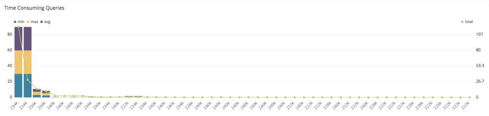
Top 50 time consuming queries:

SELECT max(query) AS max_query_id,
min(run_minutes) AS "min",
max(run_minutes) AS "max",
avg(run_minutes) AS "avg",
sum(run_minutes) AS total
FROM
(SELECT userid,
label,
stl_query.query,
trim(DATABASE) AS DATABASE,
trim(querytxt) AS qrytext,
md5(trim(querytxt)) AS qry_md5,
starttime,
endtime,
(datediff(seconds, starttime,endtime)::numeric(12,2))/60 AS run_minutes,
alrt.num_events AS alerts,
aborted
FROM stl_query
LEFT OUTER JOIN
(SELECT query,
1 AS num_events
FROM stl_alert_event_log
GROUP BY query) AS alrt ON alrt.query = stl_query.query
WHERE userid <> 1
AND starttime >= dateadd(DAY, -7, CURRENT_DATE))
GROUP BY DATABASE,
label,
qry_md5,
aborted
ORDER BY total DESC
LIMIT 50;

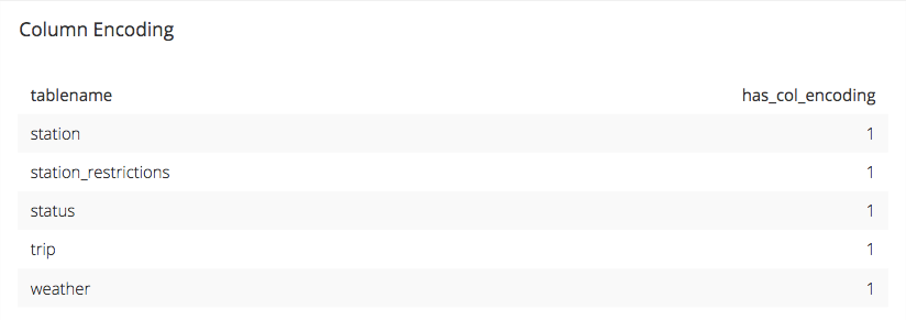
2. Column encoding

As you know Amazon Redshift is a column-oriented database. When creating a table in Amazon Redshift you can choose the type of compression encoding you want, out of the available.

The chosen compression encoding determines the amount of disk used when storing the columnar values and in general lower storage utilization leads to higher query performance. If no compression is selected, the data will be stored as RAW, resulting in a significant penalty in query’s performance.

Using the following query you can check which tables have column encoding:

Column Encoding:

SELECT "table" tablename,
CASE
WHEN encoded = 'Y' THEN 1
ELSE 0
END has_col_encoding
FROM svv_table_info ti
JOIN
(SELECT tbl,
MIN(c) min_blocks_per_slice,
MAX(c) max_blocks_per_slice,
COUNT(DISTINCT slice) dist_slice
FROM
(SELECT b.tbl,
b.slice,
COUNT(*) AS c
FROM STV_BLOCKLIST b
GROUP BY b.tbl,
b.slice)
WHERE tbl IN
(SELECT table_id
FROM svv_table_info)
GROUP BY tbl) iq ON iq.tbl = ti.table_id
ORDER BY SCHEMA,
"Table";

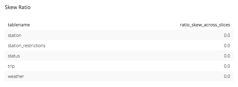
3. Skew Ratio

Being a distributed database architecture, Amazon Redshift is divided into nodes and slices, with each one of them storing a data subset.

In order to ensure your database’s optimal performance the key factor lies in the uniform data distribution into these nodes and slices. In the opposite case, you will end up with skewed tables resulting in uneven node utilization in terms of CPU load or memory creating a bottleneck to the database performance.

That being said, it is important to ensure that the skew ratio of your tables is as close to zero as possible and the following query can help you to monitor exactly this:

Skew Ratio:

SELECT "table" tablename,
100* (ROUND(100_CAST(max_blocks_per_slice - min_blocks_per_slice AS FLOAT) / GREATEST(NVL (min_blocks_per_slice,0)::int,1),2)) ratio_skew_across_slices
FROM svv_table_info ti
JOIN
(SELECT tbl,
MIN(c) min_blocks_per_slice,
MAX(c) max_blocks_per_slice,
COUNT(DISTINCT slice) dist_slice
FROM
(SELECT b.tbl,
b.slice,
COUNT(_) AS c
FROM STV_BLOCKLIST b
GROUP BY b.tbl,
b.slice)
WHERE tbl IN
(SELECT table_id
FROM svv_table_info)
GROUP BY tbl) iq ON iq.tbl = ti.table_id
ORDER BY SCHEMA,
"Table";

You can also keep track of the CPU and memory utilization of each node with the following queries.

CPU Load:

SELECT slice,
MAXVALUE
FROM svv_diskusage
WHERE name= 'real_time_data'
AND col = 0
ORDER BY slice;

Available Space:

SELECT sum(used)::float / sum(capacity) AS pct_full
FROM stv_partitions

4. Sort Keys

When using Amazon Redshift you can specify a column as sort key. This means that data will be stored on the disk sorted by this key. An Amazon Reshift optimizer will take the sort key into consideration when evaluating different execution plans, ultimately determining the optimal way.

When it comes to deciding the best key for your table you need to consider how the table data is being used. For example, if two tables are joined together very often it makes sense to declare the join column as the sort key, while for tables with temporal locality the date column. Check out more information about how to choose the best sort key.

The following query can help you determine which tables have a sort key declared.

Sort Keys:

SELECT "table" tablename,
CASE
WHEN sortkey1 IS NOT NULL THEN 1
ELSE 0
END has_sort_key
FROM svv_table_info ti
JOIN
(SELECT tbl,
MIN(c) min_blocks_per_slice,
MAX(c) max_blocks_per_slice,
COUNT(DISTINCT slice) dist_slice
FROM
(SELECT b.tbl,
b.slice,
COUNT(*) AS c
FROM STV_BLOCKLIST b
GROUP BY b.tbl,
b.slice)
WHERE tbl IN
(SELECT table_id
FROM svv_table_info)
GROUP BY tbl) iq ON iq.tbl = ti.table_id
ORDER BY SCHEMA,
"Table"

5. Table Size

Monitoring your table size on a regular basis can save you from a lot of pain. Knowing the rate at which your database is growing is important in order not to end up running out of space out of the blue.

For this reason the following query will help you settle things down and monitor the top space consuming tables in your Amazon Redshift cluster.

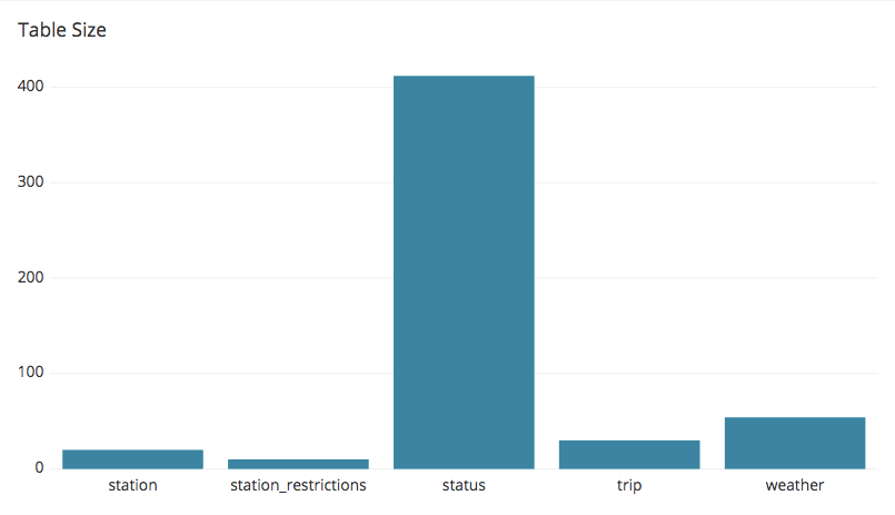
Table Size:

SELECT
"table" tablename,
SIZE size_in_mb
FROM svv_table_info ti
JOIN
(SELECT tbl,
MIN(c) min_blocks_per_slice,
MAX(c) max_blocks_per_slice,
COUNT(DISTINCT slice) dist_slice
FROM
(SELECT b.tbl,
b.slice,
COUNT(*) AS c
FROM STV_BLOCKLIST b
GROUP BY b.tbl,
b.slice)
WHERE tbl IN
(SELECT table_id
FROM svv_table_info)
GROUP BY tbl) iq ON iq.tbl = ti.table_id
ORDER BY SCHEMA,
"Table";

6. Queries Waiting on Queue Slots

In an Amazon Redshift cluster, each query is being assigned to one of the queues defined via the workload management (WLM). This means that it is possible that a query may take some time to be executed if the assigned queue is busy. As this is suboptimal, to decrease the waiting time you may increase the concurrency by allowing more queries to be executed in parallel. However, increased concurrency comes with a significant penalty in the memory share allocated to each query. When the memory share available for a query’s execution is not sufficient, disk storage will be used leading to poor performance as accessing the disk is much slower than accessing the memory.

With the following queries you can monitor the total execution time of your query and how this is divided between waiting time and actual execution along with the total number of disk based queries been executed:

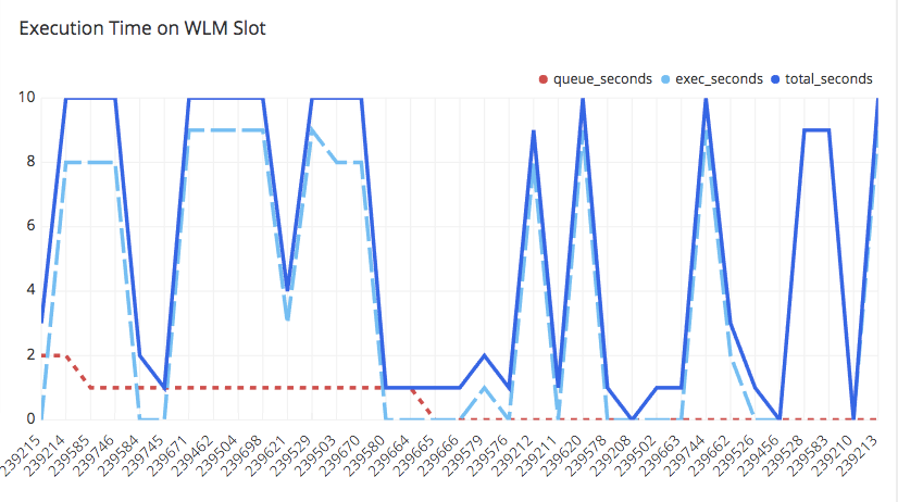
Execution Time on WLM Slot:

SELECT w.query,
w.total_queue_time / 1000000 AS queue_seconds
,w.total_exec_time / 1000000 exec_seconds
,(w.total_queue_time + w.total_Exec_time) / 1000000 AS total_seconds
FROM stl_wlm_query w
LEFT JOIN stl_query q
ON q.query = w.query
AND q.userid = w.userid
WHERE w.queue_start_Time >= dateadd(day,-7,CURRENT_DATE)
AND   w.total_queue_Time > 0
ORDER BY w.total_queue_time DESC
,w.queue_start_time DESC limit 35

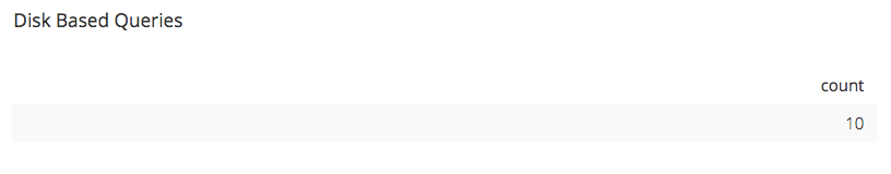
Number of disk based queries:

SELECT count(*)
FROM
(SELECT q.query,
trim(q.cat_text)
FROM
( SELECT query,
replace(listagg(text,' ') withIN
GROUP (
ORDER BY SEQUENCE), 'n', ' ') AS cat_text
FROM stl_querytext
WHERE userid>1
GROUP BY query) q
JOIN
( SELECT DISTINCT query
FROM svl_query_summary
WHERE is_diskbased='t'
AND (LABEL LIKE 'hash%'
OR LABEL LIKE 'sort%'
OR LABEL LIKE 'aggr%')
AND userid > 1) qs ON qs.query = q.query)tmp

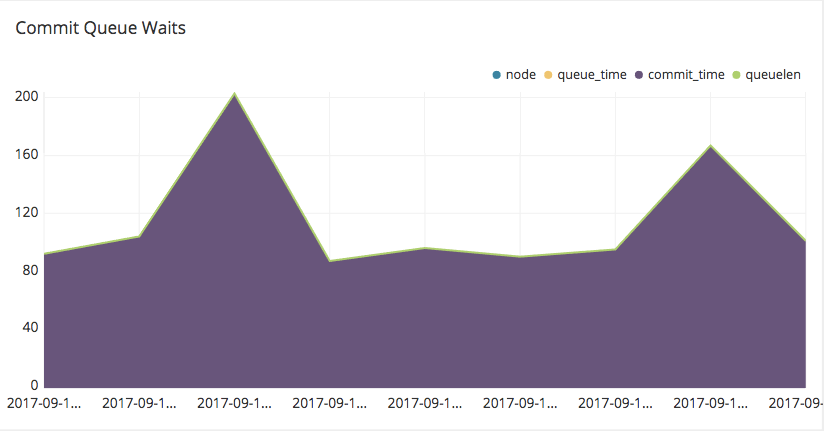
7. Commit Queue Waits

With the commit_stats.sql script provided by the AWS team you can monitor the wait time on your commit queue. As an Amazon Redshift cluster is primarily designed for the execution of analytical queries, the cost of frequent commits is terms of execution time is quite increased.

Commit queue waits:

SELECT startqueue,
node,
datediff(ms,startqueue,startwork) AS queue_time,
datediff(ms, startwork, endtime) AS commit_time,
queuelen
FROM stl_commit_stats
WHERE startqueue >= dateadd(DAY, -2, CURRENT_DATE)
ORDER BY queuelen DESC,
queue_time DESC;

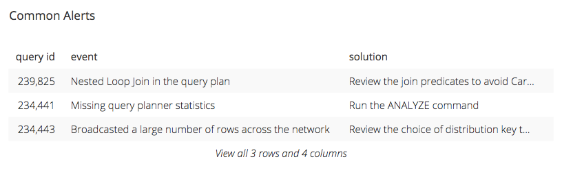
8. Finding Common Alerts

Using an Amazon Redshift cluster makes it easy to keep an eye on the most common alerts your queries produce in order to investigate them further. The following query does the trick for you.

Common Alerts:

SELECT max(l.query) AS "query id",
trim(split_part(l.event,':',1)) AS event,
trim(l.solution) AS solution,
count(*) AS "times occured"
FROM stl_alert_event_log AS l
LEFT JOIN stl_scan AS s ON s.query = l.query
AND s.slice = l.slice
AND s.segment = l.segment
AND s.step = l.step
WHERE l.event_time >= dateadd(DAY, -7, CURRENT_DATE)
GROUP BY 2,3

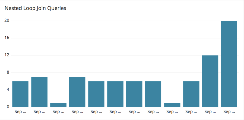
9. Nested Loop Join Queries

Investigating the most common alerts with the previously mentioned query, you may end up with a nested loop join warning.

In query execution, nested loop joins are typically a result of cross-joins. When joining two tables without any join condition then the cartesian product of the two tables is calculated. Although in cases where the outer input is small and the inner is pre indexed and large, nested joins can be reasonably effective, in general choosing them is suboptimal as their execution is computationally demanding and the penalty in performance significant.

With the following query you can monitor the number of nested loop join queries executed.

Number of loop Join Queries:

SELECT date_trunc('hour', starttime) AS
START, count(query)
FROM stl_query
WHERE query IN
(SELECT DISTINCT query
FROM stl_alert_event_log
WHERE event LIKE 'Nested Loop Join in the query plan%')
GROUP BY
START
ORDER BY
START ASC;

10. Stale or Missing Statistics

Another common alert is raised when tables with missing plan statistics are detected. During query optimization and execution planning the Amazon Redshift optimizer will refer to the statistics of the involved tables in order to make the best possible decision. For this, having tables with stale or missing statistics may lead the optimizer to choose a suboptimal plan. Defining the problematic tables with the following queries will help you proceeding with the necessary VACUUM actions.

Stale Statistics:

SELECT schema || '.' || "table" AS "table", stats_off
FROM svv_table_info
WHERE stats_off > 5
ORDER BY 2;

Missing Statistics:

SELECT count(tmp.cnt) "Table Count", tmp.cnt "Missing Statistics"
from
(SELECT substring(trim(plannode),34,110) AS plannode
,COUNT(*) as cnt
FROM stl_explain
WHERE plannode LIKE '%missing statistics%'
AND plannode NOT LIKE '%redshift_auto_health_check_%'
GROUP BY plannode
ORDER BY 2 DESC) tmp
group by tmp.cnt

11. Data Load Statistics

Regarding data loading there are best practices that the Amazon Redshift team advises users to implement. These include compressing files and loading many smaller files instead of a single huge one. Furthermore, ensuring that the number of files to load is a multiple of the number of slice results in even utilization of cluster nodes.

Some queries that help you ensure all the above are shown below.

Rows insert rate: ```sql SELECT trim(b.relname) AS "tablename",

(sum(a.rows_inserted)*1000000/SUM(a.insert_micro)) AS insert_rate_rows_ps FROM (SELECT query, tbl, sum(rows) AS rows_inserted, max(endtime) AS endtime, datediff(‘microsecond’,min(starttime),max(endtime)) AS insert_micro FROM stl_insert GROUP BY query, tbl) a,pg_class b, pg_namespace c,(SELECT b.query, count(distinct b.bucket||b.key) AS distinct_files, sum(b.transfer_size)/1024/1024 AS MB_scanned, sum(b.transfer_time) AS load_micro FROM stl_s3client b WHERE b.http_method = ‘GET’ GROUP BY b.query) d WHERE a.tbl = b.oid AND b.relnamespace = c.oid AND d.query = a.query GROUP BY 1

Scanned data (MB):

```sql
SELECT
trim(b.relname) AS "tablename",

sum(d.MB_scanned) AS MB_scanned

FROM
(SELECT query,
tbl,
sum(rows) AS rows_inserted,
max(endtime) AS endtime,
datediff('microsecond',min(starttime),max(endtime)) AS insert_micro
FROM stl_insert
GROUP BY query, tbl) a,pg_class b,
pg_namespace c,(SELECT b.query,
count(distinct b.bucket||b.key) AS distinct_files,
sum(b.transfer_size)/1024/1024 AS MB_scanned,
sum(b.transfer_time) AS load_micro
FROM stl_s3client b
WHERE b.http_method = 'GET'
GROUP BY b.query) d
WHERE a.tbl = b.oid AND b.relnamespace = c.oid AND d.query = a.query
GROUP BY 1

Scan rate (kbps):

SELECT
trim(b.relname) AS "tablename",
(sum(d.MB_scanned)_1024_1000000/SUM(d.load_micro)) AS scan_rate_kbps
FROM
(SELECT query,
tbl,
sum(rows) AS rows_inserted,
max(endtime) AS endtime,
datediff('microsecond',min(starttime),max(endtime)) AS insert_micro
FROM stl_insert
GROUP BY query, tbl) a,pg_class b,
pg_namespace c,(SELECT b.query,
count(distinct b.bucket||b.key) AS distinct_files,
sum(b.transfer_size)/1024/1024 AS MB_scanned,
sum(b.transfer_time) AS load_micro
FROM stl_s3client b
WHERE b.http_method = 'GET'
GROUP BY b.query) d
WHERE a.tbl = b.oid AND b.relnamespace = c.oid AND d.query = a.query
GROUP BY 1

Files Scanned:

SELECT
trim(b.relname) AS "tablename",
sum(d.distinct_files) AS files_scanned
FROM
(SELECT query,
tbl,
sum(rows) AS rows_inserted,
max(endtime) AS endtime,
datediff('microsecond',min(starttime),max(endtime)) AS insert_micro
FROM stl_insert
GROUP BY query, tbl) a,pg_class b,
pg_namespace c,(SELECT b.query,
count(distinct b.bucket||b.key) AS distinct_files,
sum(b.transfer_size)/1024/1024 AS MB_scanned,
sum(b.transfer_time) AS load_micro
FROM stl_s3client b
WHERE b.http_method = 'GET'
GROUP BY b.query) d
WHERE a.tbl = b.oid AND b.relnamespace = c.oid AND d.query = a.query
GROUP BY 1

Average file size (mb):

SELECT
trim(b.relname) AS "tablename",
(sum(d.MB_scanned)/sum(d.distinct_files)::numeric(19,3))::numeric(19,3) AS avg_file_size_mb
FROM
(SELECT query,
tbl,
sum(rows) AS rows_inserted,
max(endtime) AS endtime,
datediff('microsecond',min(starttime),max(endtime)) AS insert_micro
FROM stl_insert
GROUP BY query, tbl) a,pg_class b,
pg_namespace c,(SELECT b.query,
count(distinct b.bucket||b.key) AS distinct_files,
sum(b.transfer_size)/1024/1024 AS MB_scanned,
sum(b.transfer_time) AS load_micro
FROM stl_s3client b
WHERE b.http_method = 'GET'
GROUP BY b.query) d
WHERE a.tbl = b.oid AND b.relnamespace = c.oid AND d.query = a.query
GROUP BY 1

Rows inserted:

SELECT trim(b.relname) AS "tablename",
sum(a.rows_inserted) AS "rows_inserted"
FROM
(SELECT query,
tbl,
sum(ROWS) AS rows_inserted,
max(endtime) AS endtime,
datediff('microsecond',min(starttime),max(endtime)) AS insert_micro
FROM stl_insert
GROUP BY query,
tbl) a,
pg_class b,
pg_namespace c,

(SELECT b.query,
count(DISTINCT b.bucket||b.key) AS distinct_files,
sum(b.transfer_size)/1024/1024 AS MB_scanned,
sum(b.transfer_time) AS load_micro
FROM stl_s3client b
WHERE b.http_method = 'GET'
GROUP BY b.query) d
WHERE a.tbl = b.oid
AND b.relnamespace = c.oid
AND d.query = a.query
GROUP BY 1

For more expert times on how to optimize your Amazon Redshift performance, download Blendo’s white paper, Amazon Redshift Guide for Data Analysts, here.

-–

This guest blog post was written by Kostas Pardalis, co-Founder of Blendo. Blendo is an integration-as-a-service platform that enables companies to extract their cloud-based data sources, integrate it and load it into a data warehouse for analysis.