Best Practices for Developing an ELT Pipeline
Posted by on May 19, 2020 Data Governance
This is a guest post by Michael Kaminsky, founder of Kaminsky Data Strategies, which helps companies understand and implement best practices around data. Previously, Michael was the Director of Analytics at Harry’s.
Over the last few years, the work of managing and programming the way that data are stored in a data warehouse has shifted from the province of software engineers writing ETL (extract, then transform, then load) to data analysts (or analytics engineers) writing ELT (extract, then load, and transform at the end). The importance of developing data models that are easy to maintain, easy to reason about, and easy to query from has become a core competency of every data and analytics team.
With a solid ELT pipeline in place, we’ll be able to make the data and analytics team much more scalable than it was before by using software engineering best practices to write scalable and maintainable data pipelines.
In this blog post, I’m going to discuss some of the best practices for data modeling in this environment that I learned during my years running the data and analytics team at e-commerce brand Harry’s and consulting with a variety of startups developing their data platforms.
Getting Oriented
For the duration of this post I’ll be assuming you’re using something like the (now) standard ELT data stack. This generally looks something like:
- Extract and load: Stitch or Fivetran to get data from upstream sources into the warehouse
- Data warehouse: Google BigQuery, AWS Redshift, or Snowflake
- Transformation layer: dbt, Matillion, or Dataform for managing transforms
- Business intelligence tool: Chartio, Redash, Mode, Sisense, Looker, Tableau, etc. for presenting data to end users
- Downstream data consumers (maybe): Customer data platforms, machine-learning models, or other data consumers could fit into this section
You could be using a different setup, and almost all of these lessons will apply, but I’ll be showing examples assuming something like the above. If you’re doing something different, you (hopefully) have a good reason why and will know how to adjust the advice in this post to fit your needs.
Data modeling happens in the transformation layer. This is where, by applying transformations, business logic, and aggregations to the raw “source” data, the analytics team can create relations that are more useful and easier to use by downstream users and applications (e.g., analysts or BI tools).
To get oriented, I want to lay out some important terms and what they mean:
- Table: This is an object accessible in a database that has been written to disk. The act of querying a table involves reading data directly off the disk.
- View: This is an object accessible in a database that has not been written to disk. The act of querying a view involves reading data from the disk, applying the transformation logic encoded in the view, and then presenting the results from the query.
- Relation: This is used to refer to both views and tables. It’s a table-like object in a database that is queryable regardless of how it is materialized.
- Data model: This is the highest level of abstraction and includes relations as well as other intermediate objects that might not be queryable at all in the database (e.g., re-usable chunks of code that are never actually created in the database).
We use “transformations” when we’re modeling data to create relations in the data warehouse.
One easy example of a transformation that might be modeled in the data warehouse is de-normalizing data that come from a transactional database so that analysts do not have to rewrite the join logic every time they want to perform an analysis. If you’re using a SQL-based transformation tool like dbt, you might create a relation using a transformation definition that looks like this:
-- denormalized_users.sql
SELECT
    users.id AS user_id
  , users.email as email_address
  , geography.state
  , geography.region
  , geography.country
  , account.account_type
  , account.created_at as account_created_at
FROM users
LEFT JOIN geography
  ON users.id = geography.user_id
LEFT JOIN account
  ON users.id = account.user_id
If you create this relation in your warehouse, downstream users no longer have to remember where the geography data or account data are stored—they can simply query directly from the denormalized_users relation.
Of course, this is a very simple example. Most businesses require much more complicated transformations and queries to create objects that are core to measuring and running the business.
Why do we need the transformation layer?
This layer is critically important to building a data pipeline that can support the growth of your business. If you’re reading this article, you’ve probably already felt the pain of a missing transformation layer at some point in your career:
- You have to copy and paste SQL queries over and over again to reuse logic that someone (who knows who) originally wrote 18 months ago
- If the production application database schema changes, all of the dashboards and everyone’s reporting breaks, and you have to go around and fix every broken piece, and notify everyone who might be using the now-defunct snippet of code
- Your queries are tangled messes of hundreds of lines of SQL code with complicated CTEs and joins
- Making changes to any existing report is a scary and error-prone process
These types of problems indicate that there’s a missing abstraction layer that should make doing this type of software engineering work much more manageable.
We use this abstraction layer to achieve a number of goals, all of which will be familiar to software engineers working in complex systems, but may be less familiar to analysts who do not come from an engineering background.
We want to:
- Codify “agreed upon” logic in a version-controlled system that is easy to reference.
- DRY (Don’t Repeat Yourself) out our analytics codebase so that logical changes can easily be propagated to all downstream consumers.
- Expedite more complex downstream analyses by leveraging abstraction layers that facilitate higher-order reasoning with simple(r) relations and conceptual objects. That is, it’s easier to reason about a
user_cohort_valuetable than having to think about the constituentusers,orders, andsubscriptionstables. - Make analyses less error-prone by non-analyst business users or data scientists less familiar with the intricacies of the data.
Achieving these goals will help us make the analytics team much more scalable than it was before and will free up time to invest in sophisticated and value-generating analyses rather than just maintaining a fragile data pipeline.
The data-DAG
In order to add additional complexity while making use of abstractions defined previously, the transformation layer is really just a chain of transformations where raw data feed into an initial transformation and each subsequent transformation reads from transformations at a lower level of abstraction. In the computer science world, we refer to this type of chain as a Directed Acyclic Graph, or, simply, DAG. It’s “Directed” because it has a direction—from raw data to cleaned data, “Acyclic” because it cannot have transformations that are mutually dependent, and a “Graph” because it can be expressed as a network of nodes and edges.
In this post, I’ll use the terms “upstream” and “downstream” to refer to transformations at a lower and higher level of abstraction, respectively. To stay oriented, think about the flow of a data as a river running from the raw data (upstream) toward the cleaned data that are ready to be used (downstream). This diagram should help you get oriented:
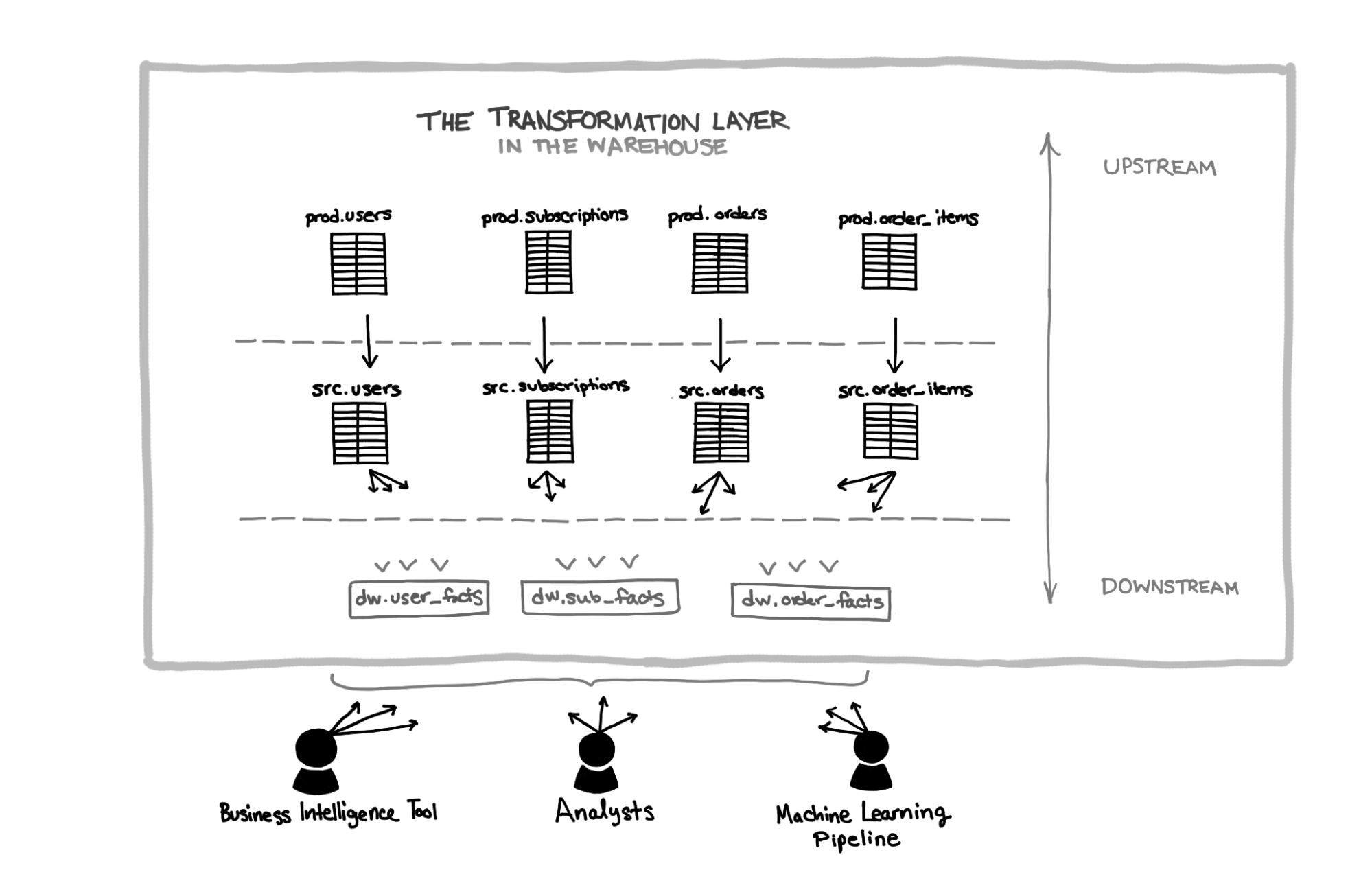
Here, the most upstream data are the tables coming directly from the production application database, copied into the warehouse without transformation. Then come the source tables that may have light transformations applied, and finally “data warehouse” tables that combine the source tables into more end-user friendly relations. Downstream applications and analysts query from the data warehouse tables without having to know about the more upstream tables and their transformations.
Again, this is a fairly simplistic example. In the real world, the data DAG might be made up of many transformations touching hundreds of upstream source tables. Fortunately, lots of great tooling exists to help manage this complexity and develop the system efficiently. dbt in particular has been a game-changer in this world as it allows for the construction and management of complex DAGs using pure SQL + Jinja templating.
Principles of Transformation
In order to make this system deliver as much value as possible to end users while remaining maintainable and extensible, there are a number of principles I recommend following when developing this system.
Use schemas to group transformations by type
Use schemas to namespace your transformations and separate them by types. Namespacing can communicate to end-users where they can find a relation they’re looking for. For example, all of the marketing-related relations can be in the marketing schema, while all of the retail-specific relations can be in a retail schema.
Namespacing by business units is common, but it could also be by abstraction level or data source. For example, you may want to group all of the transformations that use Salesforce as a datasource together. Or you may want to separate your transformations that do LTV-projection and marketing attribution from those that are doing cube-like pre-aggregations from those that are doing more straightforward data cleaning and pre-processing.
Namespacing can help developers organize the codebase to know where to look to find the logic for a given topic or abstraction.
Obey the grain
When we talk about the “grain” of a relation we mean that relation’s fundamental unit-of-analysis. A users relation has the grain of a user if each row represents a single user. In fully denormalized schemas (like in an application database) it’s generally clear what the grain of every table is. However, once we move into the world of more complex relations in a data warehouse, it becomes very important to keep track of the grain of each relation.
Here’s an example of a users relation with a grain of “user”:
| user_id | user_dob | user_email |
|---|---|---|
| 1 | 1988-01-07 | yyy@gmail.com |
| 2 | 1995-09-25 | zzz@yahoo.com |
| 3 | 1990-10-19 | alphabeta@me.com |
And here’s an example of an aggregated relation, with a grain of “state”:
| state | geo | user_count |
|---|---|---|
| texas | south | 1500 |
| california | west | 1000 |
| arizona | west | 450 |
| new york | east | 1250 |
Ideally, it should be clear from the name of the relation what the grain of the relation is—a user_weeks relation, for example might have one row per user per week. Similarly a subscription_states table would have one row per subscription per subscription-state. You get the idea.
I tend to observe grain violations in transformations written by more junior analysts who join together relations of multiple grains and then apply lots of “SELECT DISTINCT” queries to try to get down to the grain that they actually want. This code is generally difficult to read and understand, and is especially error-prone when you start layering aggregates on top of these transformations with unclear grain.
Relations with unclear grain are an indication that your warehouse transformations are not well factored and should be revised!
Use schemas to control access to different relations
In addition to namespacing to provide observational clarity as described above, you can use different schemas to provide more fine-grained access control to the relations in the warehouse. One common use-case is separating sensitive data from non-sensitive data (e.g., separating PII) and using schemas to control access to the sensitive data.
Use schemas to set your warehouse public API
In addition to limiting access for security reasons, I prefer to only provide query access for BI tools and analysts to the most downstream schemas.
This way, I know that any changes made only to upstream “intermediate” relations will not impact downstream users. That is, if changes are made to upstream or intermediate tables, I can handle them there so that the downstream schemas don’t (necessarily) have to change. This is great for handling things like column-name changes that end users shouldn’t have to be aware of. Of course, sometimes you do need to change the downstream relations, but at least you will know that potentially breaking changes are incoming and you can be responsive to them.
This is also a way of hardening the difference between the “public API” of the data warehouse that is exposed to end users and the intermediate or purely internal relations that are subject to change without notice.
Be mindful about what belongs in the presentation layer
It can be tricky to decide what logic should belong in a BI tool as opposed to what belongs in the database. I don’t have any hard-and-fast rules around this, but here are the general guidelines I use:
- Presentation layer (the BI tool):
- Simple joins used to combine relations with different grains (e.g., join users to orders)
- Simple translations purely for presentation:
- Timezone shifting
- Mapping geographic states onto geographic regions
- Title-casing strings of product names
- Data warehouse:
- Any logic that needs to be re-used across multiple different reports or relations (this is the best way to DRY out your code)
- Anything that needs to be used by multiple different downstream consumers (e.g., the BI tool, data scientists, and an ML pipeline all need access to a consistent field)
Keeping the right type of logic at the right abstraction layer can help you keep your codebase easy to read and reason about.
Code Smells
Finally, I think it’s useful to cover some of the code smells that I keep a lookout for when I’m reviewing an ELT pipeline.
These are definitely not hard-and-fast rules, but rather things to keep in mind or take a second look at. I myself have broken all of these rules while developing ELT systems, but only in times when I had a very good reason to.
Wet (not DRY) code
Familiar to any software engineer, wet code is a sign that better factoring could improve maintainability. In this workflow, DRY-ing out the code normally means moving logic upstream (i.e., “earlier” in the DAG).
One good example is date logic. Instead of copying and pasting the incantation for finding the first-day-of-the-week, I like to factor that out into one canonical calendar relation that I can just join to anywhere that I need access to the first-day-of-week variable.
Here’s an example of what that might look like:
| date | dayname | week | month | year | month_name | quarter | retail_week | retail_year |
|---|---|---|---|---|---|---|---|---|
| 2020-01-01 | Wednesday | 2019-12-30 | 1 | 2020 | january | 1 | 48 | 2019 |
| 2020-01-02 | Thursday | 2019-12-30 | 1 | 2020 | january | 1 | 48 | 2019 |
| 2020-01-03 | Friday | 2019-12-30 | 1 | 2020 | january | 1 | 48 | 2019 |
| 2020-01-04 | Saturday | 2019-12-30 | 1 | 2020 | january | 1 | 48 | 2019 |
Layer violations
If you’ve organized your data warehouse as I’ve recommended above, you’ll note that your warehouse and your DAG will begin to form “layers”; the earliest and most “raw” relations will be at the top and the latest and most “clean” relations will be at the bottom.
An important smell is if you see a relation at the downstream end of your DAG reaching deep into the upstream layers (e.g., via a join). Or, even worse, if your external consumers have to reach deep into the upstream layers. Ideally, your BI tool should only be touching the bottom-most layer of the DAG. If you find your BI tool reaching deep into the raw and untransformed layers of the data warehouse, it means that your transformations aren’t modeling all of the concepts that are important to your business and you need to do a better job of passing those through to the downstream layers.
Too many CTEs
While there are times when long, complicated queries can’t be avoided, an easy smell to identify is when there’s a transformation that has more than 3 CTEs in it. These long, complicated queries are very difficult to maintain, debug, and ensure correctness.
Factoring out some of these transformations into their own relations will make your code easier to read, and, more importantly, easier to test. (You do have an automated test suite for your transformations in place, right? If not, check out dbt and great_expectations).
In general, you want each relation to behave like a function would in an imperative programming paradigm. It should encapsulate one logical abstraction, and you should compose those different abstractions rather than trying to jam all of the logic into one big function. You should treat your warehouse relations the same way.
GROUP BY all
One smell I always look for is SQL that is frequently grouping by lots of different columns. This often indicates that the code is not obeying a consistent grain and is instead “dragging around” a lot of columns simply because they might be useful in the future.
What you want to see is code that consistently groups by the grain of the relation. If the grain is a user, you should be grouping by user_id only. If you’re consistently grouping by user_id, user_email, user_dob, etc. it probably means that your code could be refactored into separate relations or CTEs that operate at the correct grain and then join everything together at the end.
I often see something like this:
WITH

, last_week AS (
  SELECT
      user_id
    , dob
    , email
    , first_name
    , last_name
    , COUNT(order_id) AS lw_order_count
  FROM USERS
  WHERE order_created_at >= CURRENT_DATE - INTERVAL 7 DAYS
  GROUP BY
      user_id, dob, email, first_name, last_name
)

, last_month (
  SELECT
      user_id
    , dob
    , email
    , first_name
    , last_name
    , COUNT(order_id) AS lm_order_count
  FROM USERS
  WHERE order_created_at >= CURRENT_DATE - INTERVAL 30 DAYS
  GROUP BY
      user_id, dob, email, first_name, last_name
)

SELECT DISTINCT
    user_id
  , dob
  , email
  , first_name
  , last_name
  , lw_order_count
  , lm_order_count
FROM last_week
LEFT JOIN last_month
  ON last_week.user_id = last_month.user_id
When a better pattern looks more like this:
WITH

, last_week AS (
  SELECT
      user_id
   ,  COUNT(order_id) AS lw_order_count
  FROM USERS
  WHERE order_created_at >= CURRENT_DATE - INTERVAL 7 DAYS
  GROUP BY user_id
)

, last_month (
  SELECT
      user_id
   ,  COUNT(order_id) AS lm_order_count
  FROM USERS
  WHERE order_created_at >= CURRENT_DATE - INTERVAL 30 DAYS
  GROUP BY user_id
)

SELECT
    users.user_id
  , users.dob
  , users.email
  , users.first_name
  , users.last_name
  , last_week.lw_order_count
  , last_month.lm_order_count
FROM users
LEFT JOIN last_week
  ON users.user_id = last_week.user_id
LEFT JOIN last_month
  ON users.user_id = last_month.user_id
Conclusion
As with all software engineering advice, these best practices should be taken as suggestions, not as hard and fast rules. However, if you understand the conceptual ideas behind these practices—why they’re important—you’ll be well positioned to write readable, maintainable, and extensible ELT code that will increase your team’s velocity now and in the future.
Questions? Suggestions? Ideas? Drop me a line at michael@kaminsky.rocks.