Interleaved Sort Keys in Amazon Redshift, Part 2

Introduction

Previously, we discussed the role of Amazon Redshift’s sort keys and compared how both compound and interleaved keys work in theory. Throughout that post we used some dummy data and a set of Postgres queries in order to explore the Z-order curve and interleaved sorting without getting bogged down in implementation details. In this post, we will explore some of these implementation details, discuss a common tactic that can benefit from using compound and interleaved sort keys together, and run some benchmark queries against a data set with billions of rows. Throughout this post we will link to code that can be used to recreate our results.

The Zone Map: stv_blocklist

In Part I, we discussed how Redshift eschews the B-tree in favor of another secondary data structure called a zone map. The zone maps for each table, as well as additional metadata, is stored in the stv_blocklist system table. If we take a look at the definition of the stv_blocklist table, we can see it has a width of about 100B. This corresponds with our estimates from Part I regarding the small total size of this secondary data structure relative to the tables it describes.

Taking a look at stv_blocklist for a table with a compound key confirms what we’ve learned about zone maps for compound keys. Below we can see that the zone map for c_custkey, the leading column of the sort key for the orders_compound table, would prove helpful in pruning irrelevant blocks. However, the zone map for any of the other columns in the key would be useless.

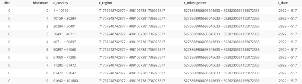
The zone map for a compound sort key (code).

If we take a look at the zone map for orders_interleaved_4, which has an interleaved sort key, we can see that the zone maps for all of the sort key columns look pretty useful.

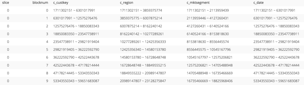
The zone map for an interleaved sort key (code).

However, it’s not the minimum and maximum column values that we are seeing here for each block but instead the minimum and maximum sort key values. Presumably, Redshift de-interleaves the zone map values on the fly whenever a query is issued in order to compare the column values in the where clause of the query to the zone map. But what’s interesting is that these sort keys don’t seem to map directly to our column values.

If we were to interleave the binary representation of the sort key column values for the first record in the table then we would expect the resulting binary value to be equal to the minimum sort key (which has a decimal value of 1,711,302,144 as shown above). However, this is not the case. Behind the scenes, Redshift is taking care of a few important details for us which we can see by examining the stv_interleaved_counts table.

The Multidimensional Space: stv_interleaved_counts

With our dummy data set in Part I, we were able to interleave the binary representation of the column values directly to produce our sort keys because we were ignoring a few details about working with real data.

Sort keys need to be represented by a data type within the database. Redshift uses a bigint to represent the sort key which is a signed 64-bit integer. However, the values of our sort key columns could be of type bigint as well. If we had four bigint sort key columns, then interleaving their bits would produce a 256-bit sort key which could not be stored as a bigint. To account for this, Redshift uses a proprietary compression algorithm to compress the values of each sort key column (this is separate from the compression encoding type of each column). These compressed values are what actually get interleaved and we can take a look at them in the stv_interleaved_counts system table.

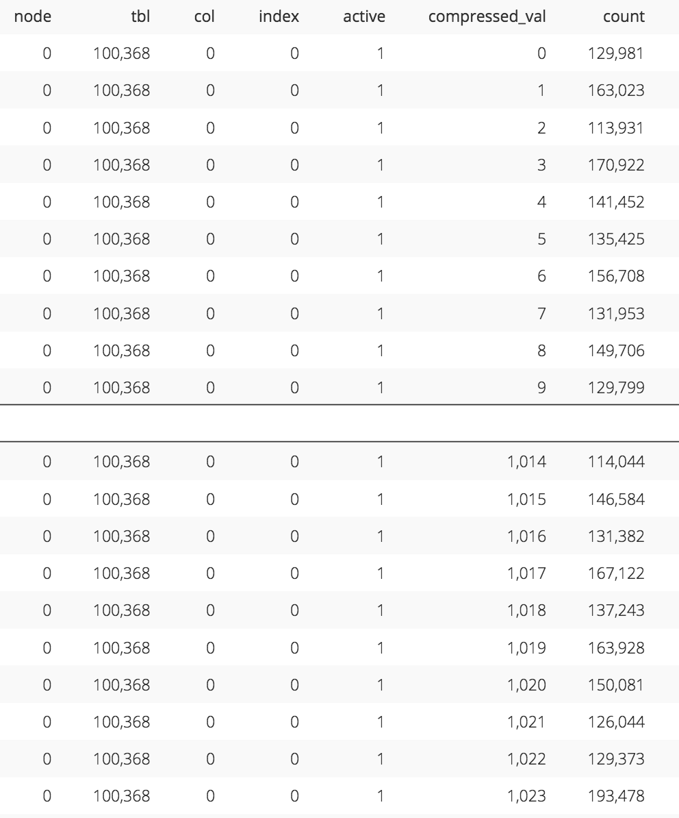
An abbreviated view of the stv_interleaved_counts system table for orders_interleaved_4 (code). Notice the the count of records assigned to each compressed_val is somewhat balanced._

We can check that it is in fact these compressed values that are being interleaved to produce the sort key by interleaving the binary representation of the minimum compressed value for each sort key column to produce the minimum sort key. Likewise, we can interleave the binary representation of the maximum compressed value for each sort key column to produce the maximum sort key.

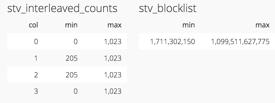
Above, the table on the left shows the minimum and maximum compressed values for each sort key column of orders_interleaved_4. On the right, we see the minimum and maximum sort key values for the entire table (code). Below, we see that if we interleave the binary representation of the values on the left above, we get the binary representation of the values on the right above._

What these compressed values ultimately represent are the dimension coordinates of the multidimensional space for which Redshift will fit a Z-order curve. The stv_interleaved_counts table gives us an idea of how this space is laid out.

The coordinate range of each dimension is constrained by the size of the sort key. Since the sort key can be a maximum of 64 bits in size, then the size in bits of the maximum coordinate of each dimension can be no more than 64/N where N is the number of columns in the sort key. For example, the range of coordinates for orders_interleaved_8, which has an eight-column interleaved sort key, is 0 to 255. This makes sense since 2^(64/8) equals 256.

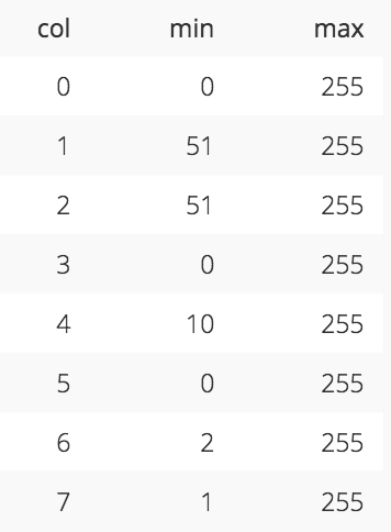
The coordinate range for each column of an eight column sort key, as seen in orders_interleaved_8, is limited to 256 values (code)._

If the sort key had only a single column then Redshift could potentially use the entire 64 bits for the maximum coordinate resulting in a range of 0 to 9,223,372,036,854,775,807. In this case, the sort should theoretically be no different than a compound key since we only have a single column. However, zone maps for compound keys only take into account the first 8 bytes of the sort key column values. If the column values have a long common prefix, such as “https://www.”, then a zone map on the first 8 bytes won’t be of much help. Redshift’s proprietary compression algorithm for interleaved sort keys does a better job of taking into account the entire column value so that different values with common prefixes get different compressed values and thus different sort keys yielding a more useful zone map.

Interestingly, as we’ve seen before, the range of coordinates for orders_interleaved_4, which has a four-column interleaved sort key, is 0 to 1,023. In this case, it looks like the coordinates are actually 10 bits in size (2^10 equals 1,024) but conceivably, they could be as large as 16 bits for a range of 0 to 65,535 (2^(64/4) equals 65,536). The reason for the smaller size is likely due to the size and distribution of the data and Redshift’s attempts to prevent skew.

Skew: svv_interleaved_columns

Interleaved sort keys aren’t free. The magic of the Z-order curve works best when data is evenly distributed among the coordinates of the multidimensional space. Upon ingestion, Redshift will analyze the size and distribution of the data to determine the appropriate size of the space and distribute the data within the space to the best of its ability. This logic is a part of the proprietary compression algorithm that maps column values to the compressed values in stv_interleaved_counts and it may need to be “recalibrated” over time to prevent skew (this is separate from distribution skew across slices). We can see a measure of this skew by looking at the svv_interleaved_columns system table.

Note: AWS will be releasing a patch that significantly improves the skew measurements in svv_interleaved_columns to better account for duplicate values. We will update the tables below with new measurements once the patch has been released.

Skew can be caused by a few different factors, some of which cannot be accounted for. Columns with low cardinality will show a degree of skew because the records will be assigned to a small number of coordinates in the dimension. Redshift will try to space these few coordinates out as evenly as possible but there will still be a lot of coordinates that are left empty. This is demonstrated by the c_region column of the orders_interleaved_4 table.

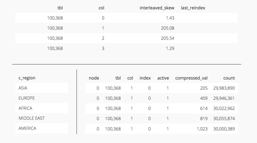
The upper table here shows the skew for each column of the sort key for orders_interleaved_4 (code). Notice c_region (column 1) has a really high skew. This is because it has a cardinality of 5 as shown in the table on the bottom left (code). Because of this, Redshift can only assign records to 5 coordinates on the c_region dimension of the multidimensional space as shown in the table on the bottom right (code).

Data that is inherently skewed cannot be accounted for either. In the orders_interleaved_skew_custkey table we’ve reassigned half of the data a c_custkey of 1. The c_custkey column still has a high cardinality in that there’s still a lot of customers but one customer dominates the data set. We can see this skews the data towards the first coordinate in the dimension.

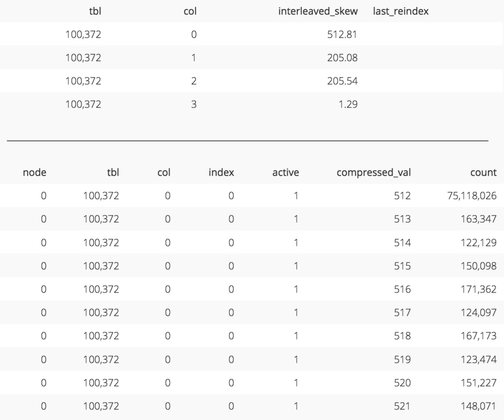
The upper table here shows the skew for each column of the sort key for orders_interleaved_skew_custkey (code). Notice c_custkey (column 0) has a really high skew. This is because the data set is dominated by a c_custkey of 1 and therefore a large number of records are being assigned to coordinate 512 on the c_custkey dimension of the multidimensional space as shown in the bottom table (code). Also note that only half of the c_custkey dimension is being used as 512 is lowest coordinate with records assigned to it.

For both of the cases above there’s no way to recalibrate the compression algorithm and resort the data to eliminate this skew. However, if the skew is artificial, meaning a large number of records are being assigned to the same coordinate when they could in fact be redistributed, then we can use the vacuum reindex command to fix this. This commonly occurs for data that increases monotonically over time, such as dates, where all values inserted after the first data load will be assigned to the last coordinate in the dimension causing artificial skew.

For example, the orders_interleaved_skew_date table was loaded with data up until 01/01/1998 on the first load. After this initial load, only the c_region and c_mktsegment columns are skewed due to low cardinality. The d_date column has a relatively low skew.

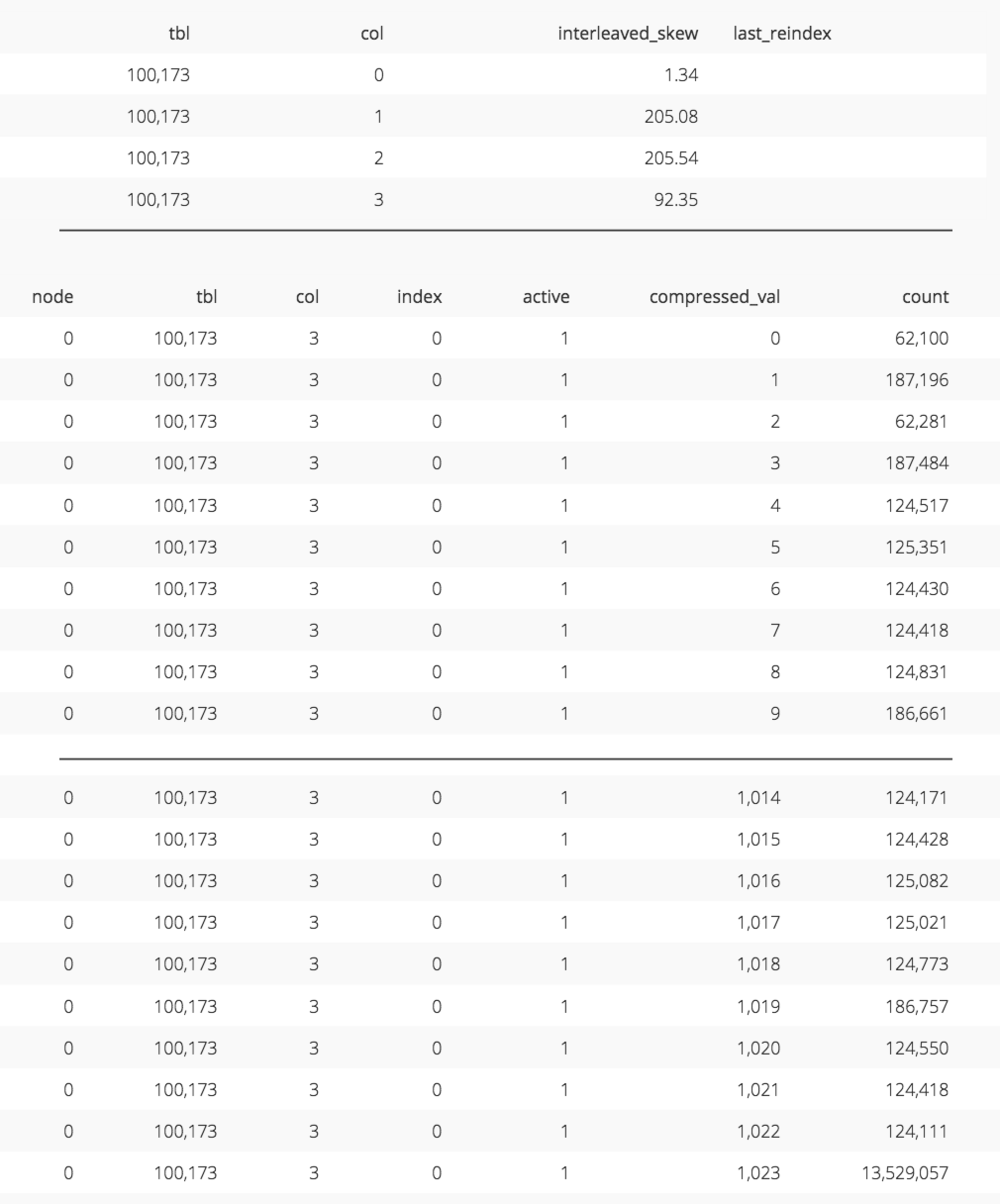
The upper table here shows the skew for each column of the sort key for orders_interleaved_skew_date after initial load (code). Notice d_date (column 3) has a low skew. The bottom table shows that records are somehwat evenly spread amongst the coordinates of the d_date dimension (code)._

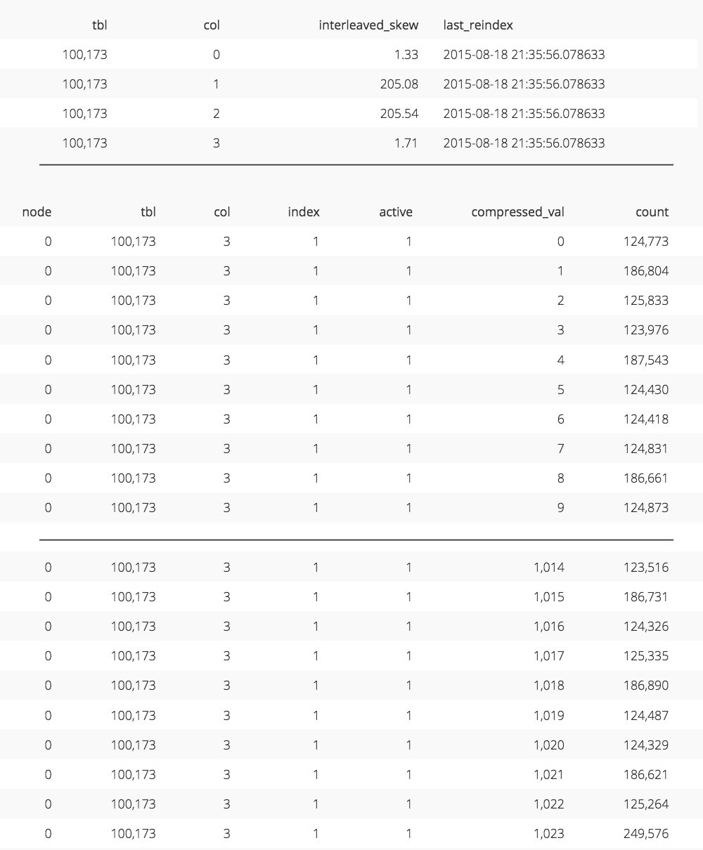
After inserting the remaining data from later than 01/01/1998, we can see the skew for the d_date column has skyrocketed because the majority of records have been assigned to the last coordinate in the dimension.

Running vacuum reindex eliminates this skew at the cost of extended vacuum times of 10% to 50% because resorting the data in an interleaved fashion potentially involves touching every storage block.

Current and Archive Tables

We can offset some of the maintenance cost associated with vacuum reindex as well as optimize for common data warehousing workloads by using compound and interleaved sort keys together in a common data warehousing design pattern; current and archive tables.

For many business processes we can assume that after a certain period of time a record is highly unlikely to be updated. For example, an e-commerce company with a return policy of 60 days can safely assume that order records over 60 days old aren’t very likely to be updated. This allows them to create an orders_current table that includes orders placed within roughly the last two months plus the current month and an orders_archive table that includes everything earlier than this window. To make this transparent to the end user they can add a view, orders_view, that uses union all to combine both underlying tables.

The goal of the orders_current table is to facilitate quick lookups of individual orders, either for pure reads or read/write operations such as update. This makes it well suited for a compound key with the order id as the leading column of the key. The goal of the orders_archive table is to facilitate historical analysis which could very well include ad hoc multidimensional analysis. This would make it well suited for an interleaved sort key on the dimensions that are most likely to be analyzed.

Using this design pattern, when the end of the current month is reached, the oldest month in the orders_current table is copied to the orders_archive table and then deleted from the orders_current table. That way the orders_archive table is likely to only be written to in an append only fashion once a month. The cost of running vacuum reindex on orders_archive would then be amortized over an entire month’s worth of data.

Benchmark

Now that we’ve seen the inner workings of both compound and interleaved keys, let’s benchmark their performance against each other with a set of 9 queries that are representative of their pros and cons. We’ll run each query 3 times on a data set of 6 billion rows (600 GB) using a 4 node dc1.8xlarge cluster and measure the average execution time. We’re not concerned with the absolute execution time here, just the relative execution time between keys for different operations.

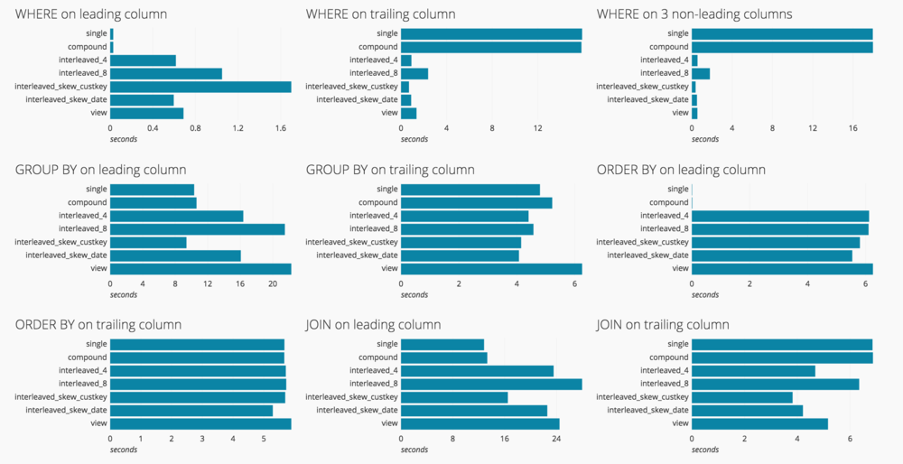
Benchmark results on 6 billion rows (600 GB) using a 4 node dc1.8xlarge cluster. The most dramatic improvements can be seen in the chart titled “WHERE on 3 non-leading columns”. orders_compound runs in about 18 seconds where orders_interleaved_4 runs over 35x faster in about 0.5 seconds.

Plotting the results shows that, generally speaking the operations tested, where, group by, order by and join, when operating against the leading column of the key perform better against a compound key. Once the leading column is excluded, the interleaved sort key performs better.

Also, as the number of interleaved sort key columns referenced in the query increases so does performance as seen by the decrease in execution time between “WHERE on trailing column” and “WHERE on 3 non-leading columns” for orders_interleaved_4. But, as the number of columns referenced in the interleaved sort key definition increases, performance decreases as seen by the increase in execution time between orders_interleaved_4 and orders_interleaved_8 for all queries.

Conclusion

Hopefully you now have a much better understanding of Redshift’s interleaved sort keys and why they are such a great fit for ad hoc multidimensional analysis. Please let us know if we missed anything as well as if you come across other interesting use cases for interleaved sort keys!