Interleaved Sort Keys in Amazon Redshift, Part 1

Introduction

Recently, Amazon announced interleaved sort keys for Amazon Redshift. Until now, compound sort keys were the only option and, while they deliver incredible performance for workloads that include a common filter on a single dimension known ahead of time, they don’t do much to facilitate ad hoc multidimensional analysis.

In Part 1 of this two-part series we will use some dummy data and a set of Postgres queries to discuss the role of sort keys and compare how both types of keys work in theory.

We won’t be performing any work in Redshift directly until Part 2, where we will examine how interleaved sort keys are implemented in practice, discuss a common tactic that can benefit from using compound and interleaved sort keys together, and run some benchmark queries against a data set with billions of rows. In both parts we will link to code that can be used to recreate our results.

Life Without the B-tree

Redshift bills itself as a fast, fully managed, petabyte-scale data warehouse and it uses techniques that you may not find in a relational database built for transactional (OLTP) workloads.

Most folks are familiar with the concept of using multiple B-tree indexes on the same table in order to optimize performance across a variety of queries with varying where clauses. However, B-tree indexes have a couple of drawbacks when applied to the large scale analytical (OLAP) workloads that are common in data warehousing.

First, they are secondary data structures. Every index you create makes a copy of the columns on which you’ve indexed and stores this copy separately from the table as a doubly-linked list sorted within the leaf nodes of a B-tree. The additional space required to store multiple indexes in addition to the table can be prohibitively expensive when dealing with large volumes of data.

Second, B-tree indexes are most useful for highly selective queries that lookup a specific data point. Analytical queries that aggregate a range of data points will typically be better served by a simple full table scan as opposed to traversing the B-tree, scanning the leaf nodes and fetching non-indexed columns from the table, as this approach suffers from a lot of random I/O, even for small ranges.

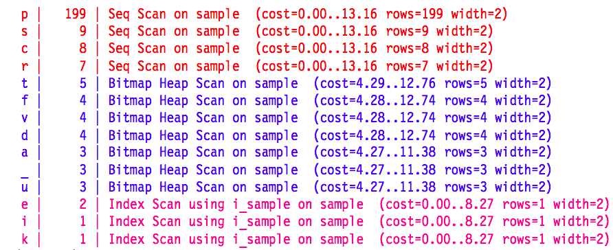
The first column here is the value being looked up in the where clause of a Postgres query, the second column is the number of records that contain the lookup value and the third column is the access method employed. Postgres’ default configuration abandons index scans pretty quickly. Bitmap scans don’t make it much further. [Source]

Compound Sort Keys and Zone Maps

For the above reasons, Redshift eschews the B-tree and instead employs a lighter form of indexing that lends itself well to table scans. Each table in Redshift can optionally define a sort key which is simply a subset of columns that will be used to sort the table on disk.

A compound sort key produces a sort order similar to that of the order by clause where the first column is sorted in its entirety, then within each first column grouping the second column is sorted in its entirety and so on until the entire key has been sorted.

This is very similar to the leaf nodes of a B-tree index with a compound key but instead of using a secondary data structure Redshift stores the data in the table sorted in this manner from the jump.

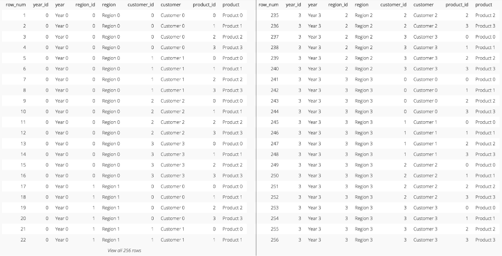
The sort order produced by a compound key on our dummy data (Get our code from GitHub). This is an abbreviated screenshot.

Once the sort order of the table has been computed, Redshift, being a columnar database breaks out each column, optionally compresses it and stores blocks of the column values contiguously on disk.

Additionally, it maintains a secondary data structure called a zone map that lists the minimum and maximum column values for each block. Since the zone map is maintained at the block level (as opposed to the row level with a B-tree), its size as a secondary data structure is not prohibitively expensive and could conceivably be held in memory. Redshift blocks are 1 MB in size, so assuming a zone map has a width of 100B, the zone map for a 1TB compressed table could be stored in 100MB.

The zone map allows for pruning of blocks that are irrelevant for any given query. If a query against our dummy data requests records where region = 2 then we can see from the zone map below that only blocks 2, 6, 10 and 14 need to be accessed.

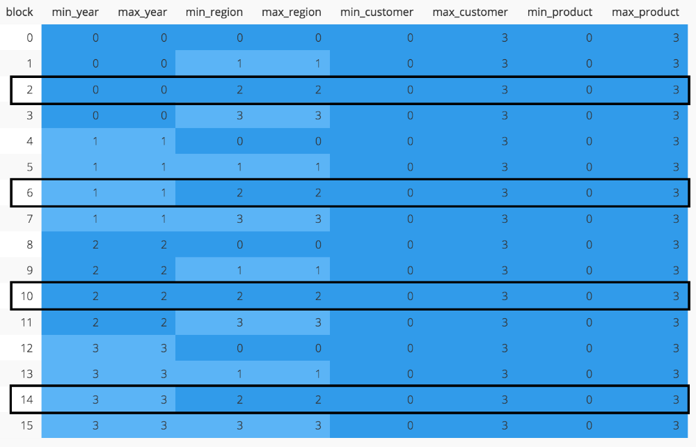
The zone map for our dummy data when using a compound sort key (code). Filtering on year or region scans 4 blocks. Filtering on customer or product scans all 16 blocks.

However, the zone map’s ability to facilitate pruning for a column depends on the sort order of the table on disk. As we can see in the zone map above, sorting on our compound key favors the leading columns in the key. An equality filter on year will scan only 4 contiguous blocks. Likewise, an equality filter on region also scans only 4 blocks, albeit non-contiguous blocks. An equality filter on customer will scan the entire table (16 blocks) because the zone map provides nothing valuable in the way of pruning. An equality filter on product must scan the entire table as well.

Another way of saying this is the compound sort key produces great locality for the leading columns of the key and terrible locality for the trailing columns. The values of the trailing columns are spread across many of the blocks in the table and any particular block includes a broad range of column values. Until recently, we either had to live with this fact or make multiple copies of the table with different compound sort keys for each. Now there’s a better way!

The Z-order Curve and Interleaved Sort Keys

To sort a table on disk we need to produce an ordered list of sort keys. A list of sort keys is a one-dimensional structure so we must linearize any multidimensional data set before mapping it to sort keys.

If we think of our data as being spread amongst the coordinates of an N-dimensional space, with N being the number of columns in our sort key, linearization would be the process of finding a path or curve through every point in this space. That path represents our ordered list of sort keys and we want it to weight each dimension equally, preserving locality across dimensions and maximizing the utility of a zone map. The sort order produced by a compound sort key represents one possible path called a row-order curve but as mentioned earlier it does a poor job of preserving locality. Luckily, the Z-order curve was introduced almost 50 years ago and not only preserves locality across dimensions but can easily be calculated by interleaving the bits of the binary coordinates and sorting the resulting binary numbers.

A 2-dimensional Z-order curve formed by interleaving the binary representations of the coordinates (x,y) and sorting the resulting interleaved binary numbers. [Wikipedia]

If we apply this technique to our dummy data the data is sorted in equal measure for both the leading and trailing columns of the key and no block stores a range broader than 50% of the column values. This means that a filter on any single column in the sort key will scan 8 out of 16 blocks.

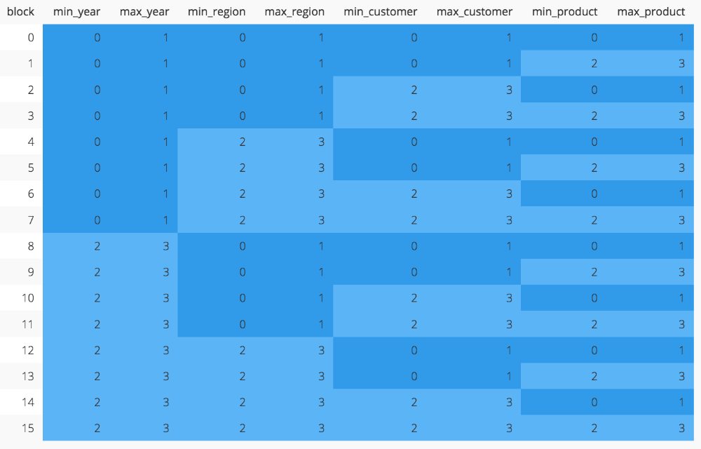
The zone map for our demo data set when using an interleaved sort key (code). Filtering on any single column scans 8 of 16 blocks.

Ideally, the number of blocks scanned for a particular where clause can be calculated as follows with interleaved sort keys:

N^((S-P)/S)

where N = the total number of blocks required to store the table, S = the number of columns in the sort key, P = the number of sort key columns specified in the where clause.

So for the 16 blocks that make up our dummy data, a four-column interleaved key results in the following block scan counts:

Filter on 1 of 4 sort key columns: 8 blocks

Filter on 2 of 4 sort key columns: 4 blocks

Filter on 3 of 4 sort key columns: 2 blocks

Filter on 4 of 4 sort key columns: 1 block

Although this suggests worse performance when filtering on the leading column compared to a compound sort key (remember we only scanned 4 blocks when filtering on the leading column of the compound key for our dummy data), the average performance across all possible sort key filter combinations will be much better with interleaved keys. This is what makes interleaved sort keys a great match for ad hoc multidimensional analysis.

The average number of block scans on our dummy data for compound vs. interleaved sort keys (code).

We can also infer two additional points from the formula above. First, the benefits of interleaved sort keys increase as the size of the data set increases. For example, if we filter on 2 out of 4 sort key columns then we scale with the square root of N and it would take two orders of magnitude in table growth before we get an order of magnitude in block scan growth.

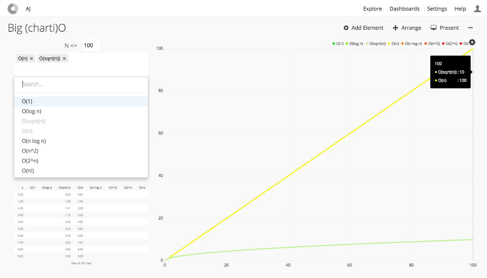
O(n) vs. O(sqrt(n))

Second, the benefits of interleaved sort keys decrease as the number of columns in the sort key increases. If instead our key was an eight-column key (which is the maximum) the block scan counts would be roughly as follows:

Filter on 1 of 8 sort key columns: 12 blocks

Filter on 2 of 8 sort key columns:  8 blocks

Filter on 3 of 8 sort key columns:  6 blocks

Filter on 4 of 8 sort key columns:  4 blocks

Filter on 5 of 8 sort key columns:  3 blocks

Filter on 6 of 8 sort key columns:  2 blocks

Filter on 7 of 8 sort key columns:  2 blocks

Filter on 8 of 8 sort key columns:  1 block

In this case, our where clause would need to be twice as robust to match the performance of the four-column key.

Conclusion

So far we’ve been speaking in terms of the ideal case and working with a dummy data set that is essentially flawless. In practice, we never get this lucky. Stay tuned for part two where we’ll dive into the implementation of these concepts in Redshift and discuss some of the considerations accounted for when applying them to real world data.

AJ Welch is a Data Engineer at Chartio.

Thanks to Russell Haering for his help in reviewing this post.

Check out part 2 of this post here.